Estimation of water resources availability - Surface water

Estimation of water resources availability is an essential prerequisite for devising efficient water resources management strategies. Assessment of water resources is not an easy task, for many reasons including the complexity and the difficult monitoring of groundwater dynamics and the limited availability of observations. Assessment of surface water resources is less complicated with respect to groundwater, for the observability of surface water bodies. Nevertheless, the rigorous quantification of river discharge and storage for natural basins is one of the most relevant challenges for water resources management.

In gauged rivers with a relatively long record of observations, estimation of water resources availability is a classical technical problem, which is usually resolved by estimating the flow duration curve (FDC). The FDC is a graphical representation, for which an analytical approximation can be provided. The use of a graphical representation presents the advantage of providing a more immediate communication to stakeholders, therefore enhancing transparency.

The FDC depicts the percentage of time (duration) over a given observation period during which a given streamflow is equalled or exceeded (see Figure 1).

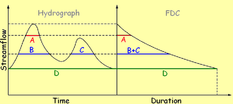
Figure 1. Construction of flow duration curve from an observed hydrograph (courtesy by Attilio Castellarin)

From a deterministic viewpoint, a FDC is a key signature of the hydrologic behaviour of a given basin, as it results from the interplay of climatic regime, size, morphology, and permeability of the basin. From a statistical viewpoint, the FDC is the cumulative probability distribution of the random variable streamflow. In fact, being the FDC an indication of the frequency (duration in relative terms) with which a given flow is equalled or exceeded, if the observation period is sufficiently long the FDC itself is an approximation of the probability of exceedance of a given river flow.

The construction of FDC from a time series of river flows observed at a given and fixed time step is straightforward. One should:

• Pool all observed streamflows in one sample.
• Rank the observed streamflows in ascending order.
• Plot each ordered observation versus its corresponding duration, in relative or absolute terms (for instance, from 1 to 365 for daily values over an observation period of one year).
• Identify the duration of the i_th observation in the ordered sample, which coincides with an estimate of the exceedance probability of the observation, 1-F_i.

If F_i is estimated using a Weibull plotting position, the duration D_i is
D_i = Pr{Q > q(i)} = 1 - i/(n + 1)
where n is the length of the daily streamflow series and q(i), i=1, 2, ..., n, are the observed discharges arranged in ascending order. The above computed FDC is called the "period-of-record" FDC.

An alternative method to compute the FDC from an observed time series is to build one FDC for each year of the observation period and then compute, for any within-year duration, the average of the corresponding river flow across all annual curves. Therefore, if the record counts years:

• y annual FDC's (AFDC) are constructed from the y-year long record of streamflows (for leap years, the streamflow measured on February 29 is discarded).
• From the group of y empirical AFDC’s one may infer the mean or median AFDC (an hypothetical AFDC that provides a measure of central tendency, describing the annual streamflow regime for a typical hydrological year)

.

• By using the same methodology adopted for inferring the median AFDC one may also construct the AFDC associated with a given non-exceedance probability p/100 (Percentile AFDC) or, equivalently, a given recurrence interval.

An example of the results from the computation of AFDC is provided in Figure 2.

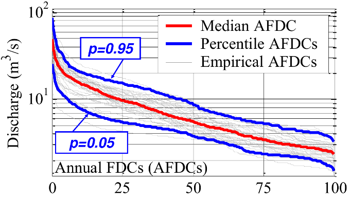
Figure 2. Construction of annual flow duration curve from an observed hydrograph (courtesy by Attilio Castellarin)

FDCs can be displayed according to different graphical representations (Figure 3).

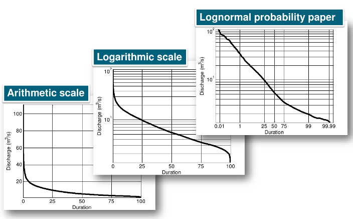
Figure 3. Graphical representations of flow duration curve from an observed hydrograph (courtesy by Attilio Castellarin)

Hitherto is was mentioned that FDCs provide a very comprehensive picture of the river regime. Figure 4 shows an example of how the different ranges of river flow can be identified.

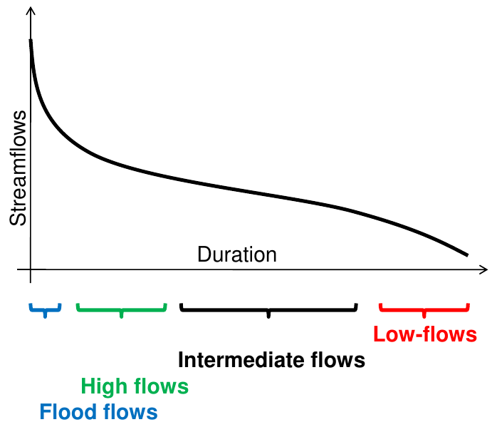
Figure 4. River flow regimes identified by the FDC (courtesy by Attilio Castellarin)

An example of graphical representation of water resources availability and functioning of a water resources management strategy through the FDC may be provided by referring to the run-of-the-river hydropower plant located at Isola Serafini over the Po River. The Figures 5, 6, 7 and 8 show the structure of the plant and the related FDC as well as other relevant variables that depend on duration.

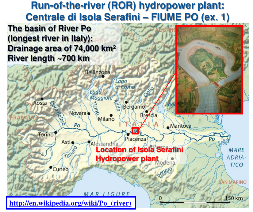
Figure 5. The hydropower plant at Isola Serafini on the Po River (courtesy by Attilio Castellarin)

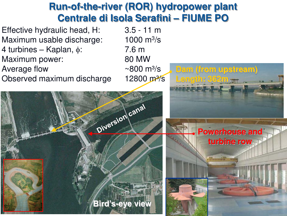
Figure 6. The hydropower plant at Isola Serafini on the Po River (courtesy by Attilio Castellarin)

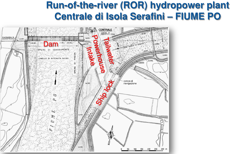
Figure 7. The hydropower plant at Isola Serafini on the Po River (courtesy by Attilio Castellarin)

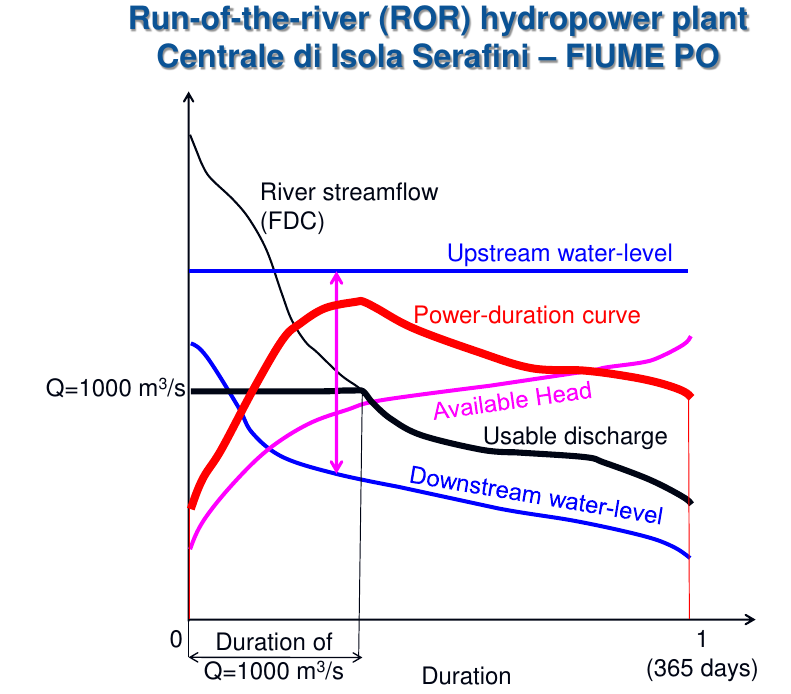
Figure 8. The hydropower plant at Isola Serafini on the Po River (courtesy by Attilio Castellarin). FDC and other relevant variables.

Estimation of FDCs for ungauged sites is a frequent technical application when designing water supply systems, ron-of-the-river hydropower plants and water withdrawals in general. It is not an easy task, for which the literature proposed several different methods.

A first possibility to reach the target is to make use of the concept of hydrological similarity. This procedure is based on comparing the considered ungauged location with a gauged location that is assumed to be hydrologically similar. Once the FDC for the gauged location is estimated, the FDC for the ungauged location is obtained by rescaling the gauged FDC of the quantity A_ug/A_g, where A_ug and A_g are the catchment areas of the ungauged and gauged location, respectively.

A second possibility is to make use of regionalisation procedure. A homogeneous region is first identified were one assumes that the FDCs for each gauged and ungauged location can be efficiently approximated by a parametric relationship. Then, optimal parameters are estimated for the gauged location and regression relationship are fitted to express the estimate parameter values depending on relevant hydrological, geomorphological and/or climatic features of the considered location. The overall procedure is then validated by reproducing the FDC for gauged locations that are treated as ungauged. An example is provided in the paper that can downloaded here.

A second possibility to estimate flow duration curves for ungauged sites, which is less applied in technical applications, is the generation of a very long record of synthetic river flow data, from which the FDC is subsequently estimated. The procedure is articulated in the following steps:

• A generation model is identified, calibrated and validated.
• The long record is generated.
• The reliability of the record is checked through a second validation procedure.
• The FDC is estimated.

A delicate issue is the reliability of the generation model. In fact, if data are generated it is likely that observation are not or scarcely available and therefore the information for calibrating and validating the model is generally limited. However, under certain situations the generation of synthetic data turns out to be useful, as the opportunity to test the design with respect to a variety of hydrological situations, which are resembled by the long synthetic record at disposal, is indeed interesting.

Rainfall-runoff models are frequently used for generating synthetic rainfall data. Their use is justified because rainfall data are more extensively available than river flows and therefore the input variables for rainfall-runoff models may be readily available for a very long period. Continuous simulation models are needed, as we need to generate a long term hydrograph. Hymod is a possible candidate, as well as more complex models.

A second class of models that is widely used for the purpose of generating synthetic river flow is formed by the stochastic processes, which are random processes.

To justify the use of a probabilistic approach for the generation of synthetic river flow data, we may recall that a hydrograph can be considered as an outcome from a collection of random variables. Let us focus on a single outcome of a river flow q(t), which occurs at time t as a realisation from the random variable Q(t). This means that the observed value q(t) is just one of the many possible outcomes. Other possible outcomes may be obtained by sampling from the probability distribution F(Q(t)). An experiment may be performed by using the following R code, under the assumption that F(Q(t)) is Gaussian with mean 100 and standard deviation 10:

prob=runif(20,0,1) #Sampling 20 random values from the Uniform distribution in the range [0-1], to be used as probabilities of not exceedance
q=qnorm(prob,100,10) #Generating outcomes from the standard normal for the probabilities above
plot(q) #Plotting the generated realisations from Q(t)

The above example makes clear that it is indeed possible to the concepts of probability to generate synthetic data. It is important to know that we generated with the above procedures several possible outcomes for a single random variable, which is the river flow at time t. To generate a hydrograph is indeed more complicated, as we need to treat each observed river flow as an outcome from its individual random variable. Therefore one needs to assume that the hydrograph is the combined realization of several random variables, each one occurring at a different time and each one governed by its own probability distribution. These random variables are generally not independent and not identically distributed. This situation is completely justified if one considers that subsequent observation of river flows have memory, if the observation time step is not excessively long. The presence of memory implies statistical dependence between subsequent observations, that the model needs to reproduce. In statistics, dependence can be reproduce through joint probability distributions. Therefore, to represent a hydrograph including nobservations one in principle needs to use a n-dimensional probability distribution to represent such collection (or family) of random variables, namely, such stochastic process. In fact, a stochastic process is defined as a family of random variables.

To reduce the above complexity, one needs to simplify the structure of the stochastic process by introducing suitable assumptions, as it is too complicate to deal with high-dimensional joint probability distributions. The idea to make the simplification is to transform the random variables through analytical relationships in order to make them independent, identically distributed and Gaussian, therefore making the process stationary, therefore describing all the outcomes by using a random variable only. The above idea sets the basis for introducing linear stochastic processes.

Linear stochastic processes are suited for modelling non intermittent processes. They assume that a series of linear and non-linear transformations can be applied to the collection of random variables to make them independent and identically distributed. The series of transformations that we are considering here is composed as follows:

• A logarithmic transformation to make the data Gaussian.
• A linear transformation to make the location parameter of the data (the mean) stationary.
• A linear transformation to remove dependence in the data, if present.

The logarithmic transformation may be operated to transform the data to resemble a Gaussian distribution. It is particularly useful in hydrology as we normally deal with positive variables. Usually the logarithmic transformation is very effective to reach the target for hydrological data, especially when they are sampled at a reasonably large time step (like daily data). After transformation a normality test should be applied to the observed and transformed sample to check whether the data are indeed Gaussian. In technical modelling strict Gaussianity may not be required, being closeness to Gaussianity sufficient for most of the real world applications. However, strictly speaking one should also check the normality of the marginal distribution of each single random variable. The latter test is rarely applied in practice. There are several alternative transformations that can be used if the logarithmic one turns out to be not successful. In what follows, we assume that the distribution of the process is multivariate Gaussian.

Deseasonalisation is usually operated to stabilize the mean of the single random variables. It can also be applied to stabilize the variance, if the process is still heteroscedastic after the logarithmic transformation. Deseasonalisation of the mean is operated by subtracting from each random variable a term that assumes different values within the yearly period but is constant from year to year. For instance, when working with daily variables deseasonalisation of the mean is operated by subtracting from each variable the daily mean. Namely, when working with an observed series, from each observation collected on Jan 1st the expected value of all the observations collected in the same day is subtracted. After the deseasonalisation, each variable will be characterised by 0 mean.

Likewise, deseasonalisation of the variance of a time series is operated by dividing each variable by the daily standard deviation, i.e., each observation collected on Jan 1st is divided by the standard deviation of all the observations collected in the same day. After the deseasonalisation, each variable will be characterised by unit variance.

In mathematical terms, let's suppose that the observed (after the logarithmic transformation above) series is indicated with the symbol Q(t,j) and the deseasonalised series with the symbol Q_d(t,j), where t is a progressive time index and j, 1 j ≤ 365, indicates the day of the year when the observation was collected. If we indicate with the symbols μ(j) and σ(j) the mean and standard deviation of the variable that refers to day j, the deseasonalised series is given by
By computing the integral in the latter relationship one obtains:

Removal of dependence is necessary to ensure that the random variables that form the stochastic process are independent. The presence of dependence can be detected by estimating correlation among the considered variables. Correlation is a measure of statistical dependence. It is estimated by computing the Pearson's correlation coefficient. Plotting the correlation coefficient against the lag time one obtains the autocorrelation function.

The literature proposed several linear transformations to remove dependence. The autoregressive model is widely used. For a zero-mean process, it can be written as

where the parameters Φ are autoregressive coefficients and ε is an independent Gaussian random variable.

The autoregressive transformation is a particular case of a more class of linear transformation, namely, the autoregressive moving-average models, also called Box and Jenkins models. They provide a parsimonious description of the memory structure of a linear Gaussian process.

If the linear transformation was successful to remove dependence, the sequence of the ε(t) should be independent, zero-mean and normally distributed. Therefore the user is readily provided with means to detect whether the linear model provides an appropriate representation of the memory of the process. Therefore, to summarize the checks that the user should make to verify model's reliability:

• Check whether the time series is Gaussian after the log-transformation.
• Check whether the series is no more periodic after deseasonalisation. To this end, the autocorrelation function is a useful tool. In fact, periodicity in the data implies periodicity in the autocorrelation function, with the same period. Therefore one should plot the autocorrelation function up to the one-year lag and check whether there is a peak.
• Check whether the series of the ε(t) is Gaussian, zero mean and independent after the linear transformation.

Further checks can be performed to check the reliability of the simulated series. These will be discussed here below.

Generation of synthetic series is carried out by reverting the transformations that were applied to the given time series to obtain the independent and identically distributed series ε(t). Accordingly, one first generates a synthetic sequence of sample size N_g of ε_g(t), where g stands for "generated". Given that these data are Gaussian and independent, they can be generated as outcomes from a Gaussian distribution with zero mean and standard deviation as the sequence of the ε(t). Then, one applies back the linear transformation, adds back the seasonal component and finally takes the exponential transformation to obtain a synthetic replicate of Q(t).

As a final step, it is advisable to carry out simple checks on the representativeness of the synthetic series, by first comparing probability density distribution and autocorrelation function for observed and simulated data. Then, one may want to compare high and low flows, and other interesting features.